

Summary
Modern vision-language-action models (VLAs) predict actions in chunks, but each new chunk starts from a stale observation, causing visible shaking at chunk boundaries. We traced this problem back to three compounding delay sources, measured each via system identification, and shifted the training target to compensate. The result was a 64.9% reduction in velocity discontinuity and a 30.8% reduction in acceleration jerk on a real bi-manual robot at 30 Hz, with no additional inference cost.
The problem: why is our robot shaking?
VLAs take camera images, joint states, and language instructions as inputs to produce motor commands. A single forward pass through a billion-parameter model takes 50–135 ms on an RTX 5090 GPU, but a manipulator needs new commands every 33 ms (30 Hz).
Action chunking helps: instead of predicting one action per step, the model predicts a horizon of 50 future actions at once. The robot executes this action chunk while the next one is being computed. This eliminates the timing bottleneck, but it introduces a new artifact.
Every time a new chunk arrives, the robot switches from one independently predicted trajectory to another. Because each chunk is conditioned on a different (and slightly stale) observation, the trajectories disagree at the boundary. The robot jerks.
The root cause: three delay sources
Most prior work treats latency as a single number: model inference time. In practice, we identified three distinct delay sources that compound:
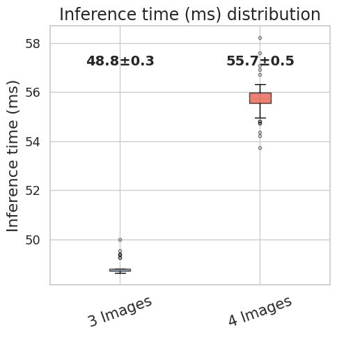
- Model inference delay, dinf (3 images = 55 ms, 4 images = 71 ms). The time for a forward pass including flow-matching denoising steps. On our RTX 5090, the model inference delay is ~71 ms with four camera images and 10 denoising steps, and ~55 ms with three images.
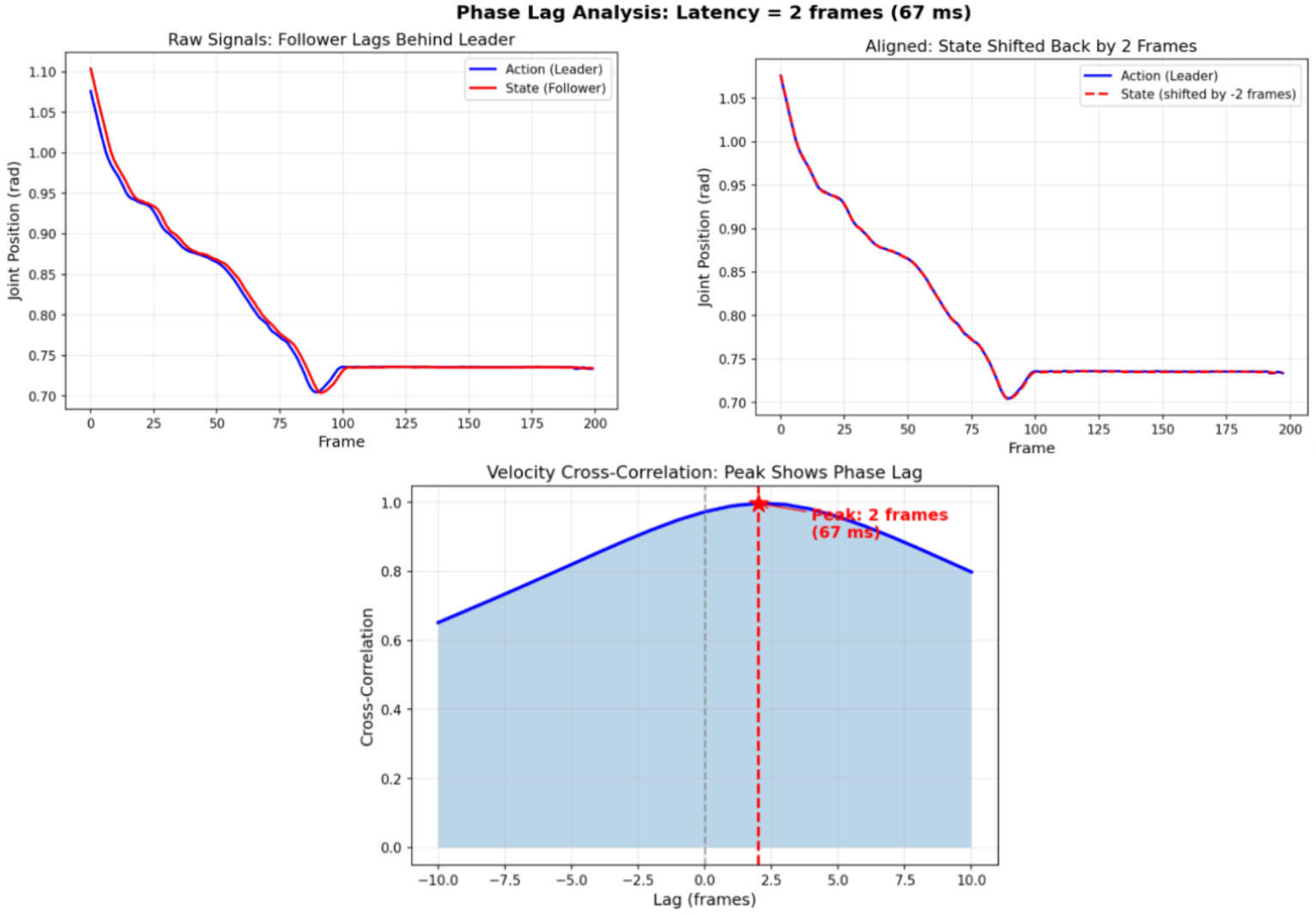
- Leader-follower mechanical lag, dlf (~67 ms). During teleoperated data collection, the follower robot tracks the leader with a ~67 ms delay due to communication latency, servo response, and mechanical compliance. The recorded joint state is always behind the commanded action. This systematic mismatch is inherent the training data.
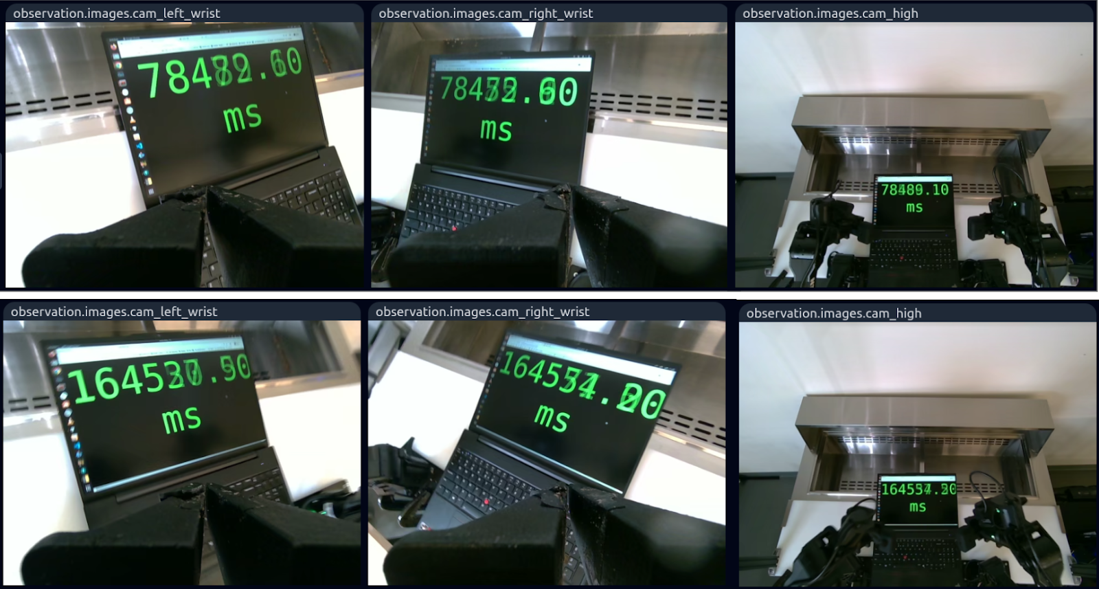
- Camera asynchrony, dcam (5-30 ms). USB cameras nominally capture at 30 Hz, but OS scheduling and bandwidth contention introduce per-camera jitter. The observation used for inference can be stale by an unpredictable amount.
The total delay seen by the policy is:

At 30 Hz, this composite delay amounts to roughly d = 3 ± 2 control steps. The standard training setup ignores this entirely. The model learns to predict actions aligned with the observation time, but at deployment, once those actions start executing, they are already obsolete. Two problems arise:
- Trajectory discontinuity. Successive chunks are conditioned on different observations, so they disagree at the boundary, producing visible shaking.
- Train-deploy mismatch. The policy is trained without delay but deployed with delay, so the observation-action alignment at test time differs from that at the time of training.
Our approach: shift and augment
The fix to this problem involves two parts: (1) shift the prediction target by the measured composite delay, and (2) augment training data with realistic time-lag perturbations for the stochastic delay components.
1. Shift the prediction target
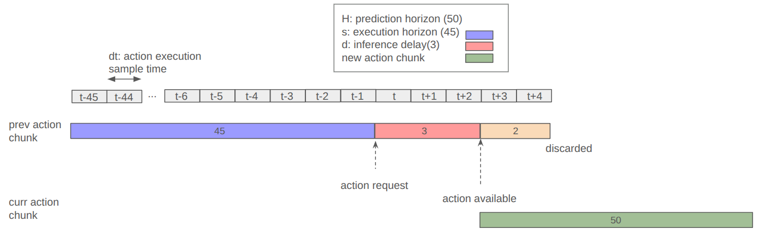
Instead of training the model to predict the action chunk starting at the current time, we shift the target action chunk forward by the measured composite delay d:

where A indicates the predicted action chunk, ot is an observation (image and joint state) at time t, and l is a prompt. H = 50 is the action horizon and d is the composite delay in control steps (e.g., d = 3 at 30 Hz ≈ 100 ms). The chunk is split into:
- Prefix At : t+d : ground-truth actions already committed (non-noisy)
- Postfix At+d : t+H : actions to be denoised by the model
2. Data augmentation for stochastic delays
The mechanical lag and camera jitter vary from step to step. A deterministic offset cannot capture this. We add two augmentations during data preprocessing:
- Follower joint-state lag injection. Replace the recorded follower joint state qtfollw with qt−dlffollw, where dlf is drawn from the empirically measured delay profile (normal distribution). This forces the policy to cope with a range of observation-action misalignments.
- Camera timestamp perturbation. Apply a random temporal offset dcam ~ ℳ(5 ms, 30 ms) to each camera’s image timestamp independently, selecting the nearest frame that is older than nominal.
In total, the composite delay used during training is d=dinf+dlf+dcam where dinf is drawn from a weighted discrete distribution over measured inference times, and the lag terms are sampled from their respective empirical profiles.
3. Modified training loss
We use conditional flow matching with per-token timesteps, allowing our model to generate action chunks individually step-by-step. We also use train-time prefix action conditioning, allowing our model to learn by giving it partial prefix action chunks as context during learning. The flow-matching loss is computed only over the postfix (actions from index d onward), and the prefix tokens are treated as fully denoised (τ=1.0). In other words, we give our model the first part of an action chunk as ground truth and only train it to generate the remaining actions:

Inference pipeline
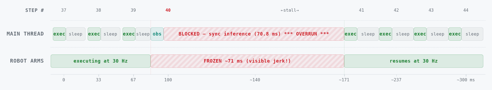
At inference time, we keep requesting action chunk predictions and execute them one after the other. This is referred to as synchronous inference, but it causes a blocking period that stops motion.
Instead of blindly waiting until a prediction is obtained, asynchronous inference issues a new request earlier, before all action chunks are carried out.
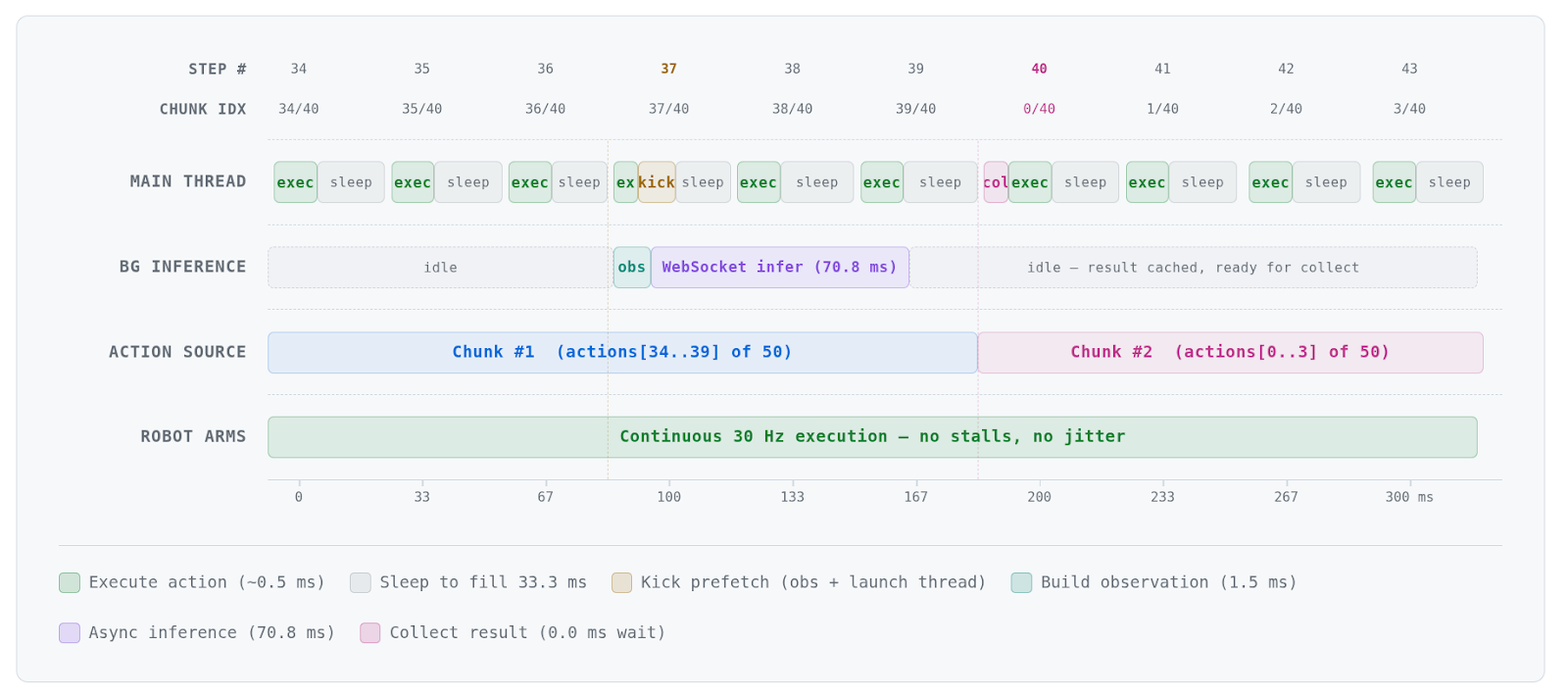
The following figure illustrates a concrete scenario with specific parameters:
At test time, the next chunk is requested d steps before the current one expires. The new chunk’s first d actions overlap with the previous chunk’s tail (the shared prefix) so that the transition is seamless. There are no backward passes or additional sampling—just standard forward inference.
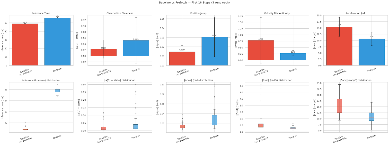
Why async prefetch alone is not enough
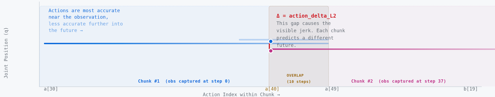
Prefetch solves the timing problem; inference finishes before the current chunk expires, so the robot never stalls. It does not solve the content problem. Each chunk is still an independent prediction from a different observation. The L2 gap between consecutive chunks persists.
Our training-time target shift forces consecutive chunks to agree on the prefix (the already-committed actions), which directly eliminates the seam.
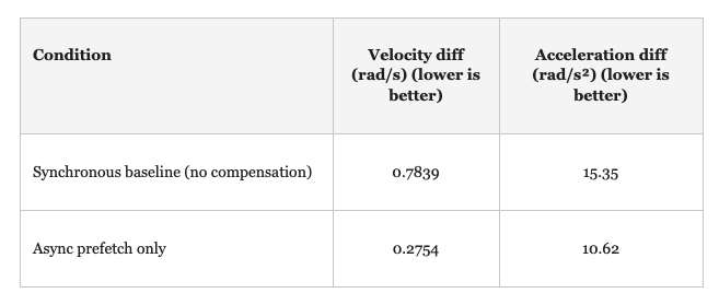
Results
We evaluate on a bi-manual Trossen robot platform running at 30 Hz with H = 50 (prediction horizon) and s = 45 (execution horizon). We estimate the velocity diff at the tail and head of consecutive chunks via first-order finite differences and similarly for acceleration diff. We compare two conditions:
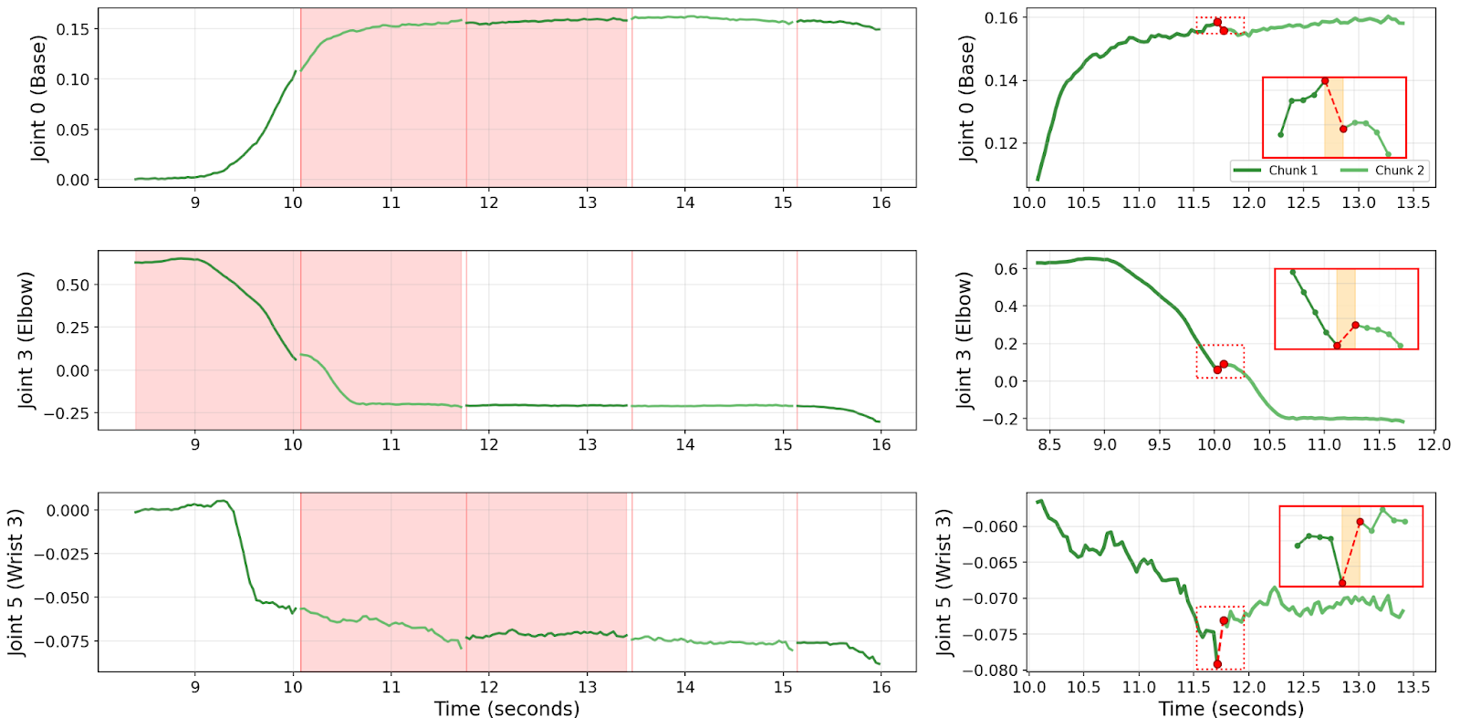
Qualitative results: wrist servo trajectory
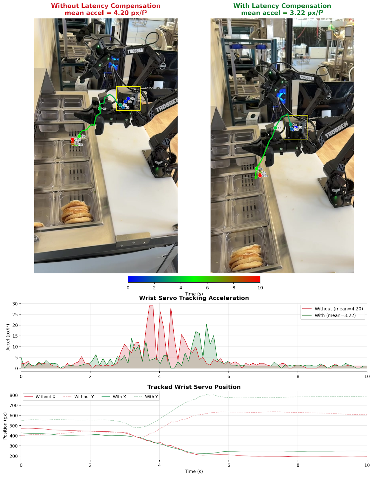
Mean pixel acceleration drops. The acceleration spikes at chunk boundaries (exactly where two independently predicted chunks disagree) disappear with our method.
Relationship to prior work
Several concurrent methods address real-time VLA execution: RTC, Training-Time Action Conditioning, A2C2, VLASH, Delay-Aware Diffusion Policy, Legato, Masked Action Chunking, and Xiaomi-Robotics-0. These methods generally model latency primarily as model inference time, which may cause inferior results, mainly due to compounding errors or out-of-bounds predictions.
Our contribution is orthogonal: we decompose the delay into three independently characterized sources (inference, mechanical, camera) and address each with a targeted strategy. This means our approach can be combined with any of these methods (which are not aware of delay compensation) for superior results.
Conceptually, the approach is a learned Smith predictor (i.e., a control system with a significant feedback time delay). Instead of building an explicit forward model, the VLA implicitly learns to predict actions that account for the expected future state of the robot, because it was trained with the appropriate delay offset. The time-lag augmentations play the role of robust control under delay uncertainty.
Limitations
- Fixed delay assumption. The delay distribution is set from system identification and does not adapt online. Hardware changes (e.g., a different GPU or a different network) require re-profiling.
- Stationary delay model. We assume the delay distribution is stable, but GPU thermal throttling and USB bandwidth drops can shift it over time.
- Single-task evaluation. Validated on one platform and task class. Generalization to different robots and manipulation scenarios remains to be tested.
Takeaway
Before adding complexity to the model or the inference pipeline, measure the delays in your system and train against them. Three simple changes—a target shift driven by system identification, follower-lag injection, and camera-timestamp perturbation—cut chunk-boundary jerk by 64.9% on our real robot, with zero inference overhead.
Contributors
Inkyu Sa, Xiaoyi (Sherry) Chen
%20copy.png)

.png)